It goes without saying that the field theory is one of the most promising utilities in physics, while there are few volumes which really concentrate on it. So I write this article just for a kind of supplement. Readers should notice this post includes classic field theory alone without relativity, and if you want know more about quantum field theory, please let me know.
Introduction
As far as I am concerned, the first man who introduced the idea of the field is Michael Faraday who developed the idea of electromagnetic induction, to describe electric lines. It is sorry that he did not make any concrete progress, mainly because of his lacking of Mathematics education. Later on, the significant triumph of the field theory was realized by James Clerk Maxwell for the famous Maxwell Equations. In the mean time, the gravitation as well as hydrodynamics were keeping up with those milestones, developing their field theory, especially the hydrodynamics due to the similarity. Till now, electromagnetism, together with hydrodynamics(fluid dynamics) is the most active area of the field theory.
A classical field theory is a physical theory that describes the study of how one or more physical fields interact with matter. Any physical field can be thought of as the assignment of a physical quantity at each point of space and time. For example, in a weather forecast, the wind velocity during a day over a country is described by assigning a vector to each point in space. Each vector represents the direction of the movement of air at that point. As the day progresses, the directions in which the vectors point change as the directions of the wind change. From the mathematical viewpoint, classical fields are described by sections of fiber bundles (covariant classical field theory).
Let us come straight to the point and start with three simple but essential concepts:
The Gradient
The gradient (or gradient vector field) of a scalar function 


where 

where 
As for the gradient of a vector field, things are getting complicated. For a trivial three-dimensional rectangular coordinates, it is defined by:
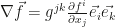
where 

The Divergence
The preliminary concept of divergence is introduced by vector calculus, noting as


where f is a given vector field. More rigorously, the divergence of a vector field F at a point p is defined as the limit of the net flow of F across the smooth boundary of a three-dimensional region V divided by the volume of V as V shrinks to p. Formally, it is defined as following:

where |V| is the volume of V, S(V) is the boundary of V, and the integral is a surface integral with n being the outward unit normal to that surface. The result, div F, is a function of p. From this definition it also becomes explicitly visible that div F can be seen as the source density of the flux of F.
A more common description is in Cartesian coordinates:
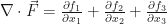
where 
The Curl
The curl of a vector field F, denoted by curl F, or ∇ × F, or rot F, at a point is defined in terms of its projection onto various lines through the point.If 

Likewise, the curl in Cartesian coordinates is most popular:

Interestingly, it also can be converted into a determinant, but we are not going to write in here for simplicity.
Thanks to the symmetry, for I am able to copy and paste to save my poor eyes!
